JPlotter
 Download JPlotter
Version 2.0 • English • Windows (32 Bit)
All files and versions
Download JPlotter
Version 2.0 • English • Windows (32 Bit)
All files and versions
Contents:
⇑
Simply download for Windows 32 Bit
or Windows 64 Bit and extract the zip archiv.
There is a file JPlotter.jar and rechne.dll.
Make sure that rechne.dll is next to JPlotter.jar when starting. Execute JPlotter.jar (requires JRE) via double click or with the following command:
What is rechne.dll?
rechne.dll is the dynamic Windows library from the rechne.exe project.
This library allows for the computation of arbitrary mathematical terms.
This library does the actual calculation of the functions values while JPlotter itself only does the plotting and GUI functions.
The program main window is strutured as follows:
⇑
Open the menu y=f(x) and add a new function. 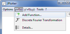
How does plotting work?
For each function a number of samples is calculated. The distance between two samples can be set in the settings menu (default is 2 pixel).
Beginnig from the left x border each 'x' character in the function gets replaced by the decimal value of x. This term gets passed to rechne.dll
which returns the y value for this sample. After the y values for all samples are calculated the points are going to be plotted.
⇑
⇑
The difference between the modes can best be explained with the function `sqrt(x)` in the interval `[-5;5]`:
`Re{f(x)}` and `Im{f(x)}` are both real functions and can be plotted separately.
`sqrt(x)={(sqrt(x)+i*0,if x>=0),(0+i*sqrt|x|,if x<0):}` therefore `Re{sqrt(x)}={(sqrt(x),if x>=0),(0,if x<0):}` and `Im{sqrt(x)}={(0,if x>=0),(sqrt|x|,if x<0):}`
For `x<0` the real part is `0`. The imaginary part is `sqrt|x|`. For `x>=0` the real part becomes `sqrt(x)` and the imaginary `0`.
Again `|f(x)|` and `arg(f(x))` are two real functions which can be plotted separately.
`|sqrt(x)|={(sqrt(sqrt(x)^2+0^2)=sqrt(x),if x>=0),(sqrt(0^2+sqrt|x|^2)=sqrt|x|,if x<0):}` and `arg(sqrt(x))={(arctan(0/sqrt(x))=0,if x>=0),(arctan(sqrt|x|/0)=arctan(oo)=pi/2,if x<0):}`
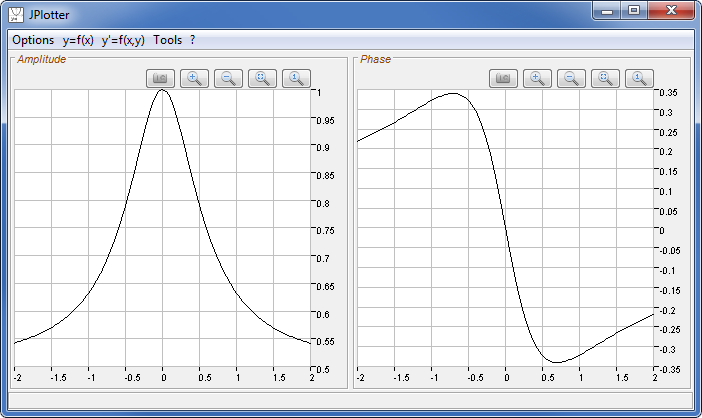
The amplitude goes over the complete interval and is mirrored at the y-axis. For `x<0` The phase is `pi/2` because the imaginary part is non-zero while the real part equals zero. For `x>=0` the phase is `0` (as for normal real numbers).
Plot of Amplitude and Phase:
The math behind it:
`f(x) = (1+i*x)/(1+2*i*x) = (sqrt(1+x^2) * e^(i*arctan(x)))/(sqrt(1+(2x)^2) * e^(i*arctan(2x))) = sqrt((1+x^2)/(1+(2x)^2)) * e^(i*(arctan(x)-arctan(2x)))`
where `sqrt((1+x^2)/(1+(2x)^2))` is the amplitude function and `arctan(x)-arctan(2x)` is the phase function. Those two functions are real now. If you plot them separately you will get the same graphs as above.
⇑
JPlotter allows for performing a Discrete Fourier Analysis on all functions currently plotted.
The Discrete Fourier Transform (DFT) of a function `f(x)` is `F{f(x)}`. The point-wise calculation
of the Fourier transform is:
`X_k=sum_(n=0)^(N-1)x_n*(cos(-2 pi k n/N)+i*sin(-2 pi k n/N))` for point number `k` of a total of `N` function points (`k,N in ZZ`).
The resulting plot is:
For `cos(x)`:
Fourier transform is real only with two positive peaks at the beginning and ending of the interval.
For `sin(x)`:
Fourier transform is imaginary only with one positive peak at the beginning and one negative peak at the ending of the interval.
The math behind it (for continuous functions):
For further examples on DFT see rectangle / unity step function and Dirac Impulse in the following section.
⇑
These functions can only be added by the use of the wizard. There is no way of typing them as a f(x) function.
Example of a non-periodic rectangle function with Discrete Fourier Analysis:
Let's check the inverted case:
Example of a periodic sawtooth function and unity step functions:
Example of a unity step function with its Discrete Fourier Transform: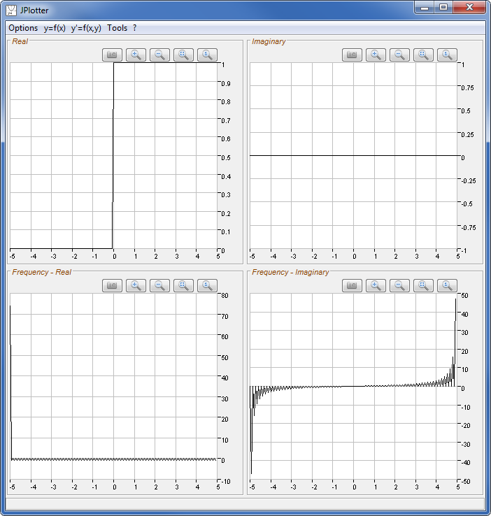
Only the quadratic spline interpolation produces a continuous function. All other interpolation techniques produce separate
functions between two or three points.
Hints for the input:
⇑
Example:
Example:
Some examples:
In case of complex functions:
Real and imaginary part are derived separately.
Example:
How does integrating work?
Real and imaginary part are integrated separately.
In case of complex functions:
Real and imaginary part are mirrored separately.
Example:
In case of complex functions:
Real and imaginary part are shifted separately.
Examples:
Examples:
How does area calculation work?
Between two sample points the area of a trapeziod is calculated. The shorter the distance between two samples the more precise it is.
Finally the area of all trapezoids is summed up. Of course this method is only an approximation to the real value.
The area calculation between a function and a derivative is less precise because the derivative function is always one sample shorter than the original function.
Keep in mind that this way areas are always positive! For example the area of `sin(x)` from `-pi` to `pi` is `2` and not `0`.
Example: `y=e^-x * sin(10x)` within `[0; 5]`:
⇑
Since phase portraits are no 'real' functions (in a mathematical manner) and slope (on y-axis) / y value (on x-axis) do not fit into a normal x/y coordinate system, they are always plotted in a separate window.
Example 1: phase portrait of `y=sin(x)` within `[0 ; 2 pi]`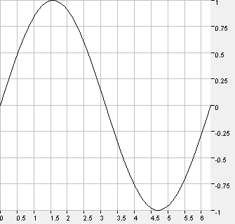
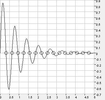
Example 2: phase portrait of `y=e^-x * sin(10x)` within `[0 ; 4]` 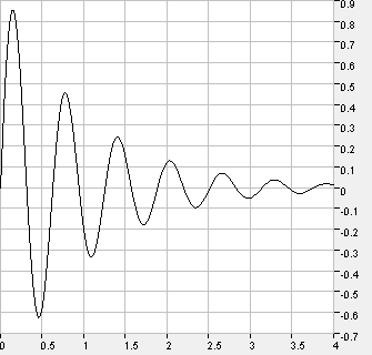
⇑
Let's look at the math for an analytical solution:
`y' = dy/dx = x*y -> dy/y = x dx -> int 1/y dy = int xdx -> lny = 1/2x^2 + C^** -> y = e^(1/2x^2+C^**) = C * e^(1/2*x^2)`
If you follow the little lines across the canvas you will find many possible courses of functions that would match the
differential equation. This is because of the unknwon variable `C`.
It seems the slope lines represent some kind of parabolic function (similar to `x^2`).
How does plotting of directional fields work?
Within the area specified (in our example above `[-3;-3]` to `[3;3]`) a grid of points gets allocated.
The upper left point has the coordinates `[-3;-3]` the point right next to it `[-2.9;-3]`,
the point below it `[-3;-2.9]` and so on. Afterwards the coordinates of each point get applied to the function `f(x,y)`
and the return value is `y'` which is the slope at this point.
The slope can be plotted as a little line with the function `slope * x`.
⇑
Some examples:
Hints for the input:
Some examples:
Examples:
Hints for the input:
Example:
Hints for the input:
Settings / Options for Rechne Console:
List of functions/operations:
⇑
JPlotter and its sources are published under the
GNU General Public License (version 3).
Feel free to use, copy or edit JPlotter under the terms of this license.
Please note: As stated in GPL JPlotter comes with absolutely no warranty.
rechne.dll and sources from the rechne.exe project are GPL as well.
Installation
Make sure that rechne.dll is next to JPlotter.jar when starting. Execute JPlotter.jar (requires JRE) via double click or with the following command:
java -jar JPlotter.jar
What is rechne.dll?
The program main window is strutured as follows:
 |
|
Getting started
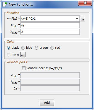
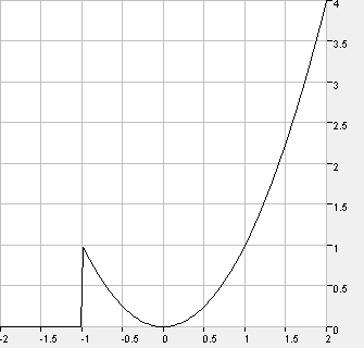
| In the following example the function `(x-1)^2-1` will be plotted for the interval `[-2;3]`.
Note the following rules for functions:
The resulting plot is: 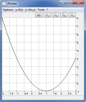
|
 |
| Multiple functions can be added to the same canvas. If another function is added the x bounds are now fixed but they can be changed in the settings menu. Adding `sin(x)` to the canvas the resulting plot is: 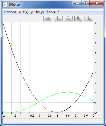
|  |
How does plotting work?
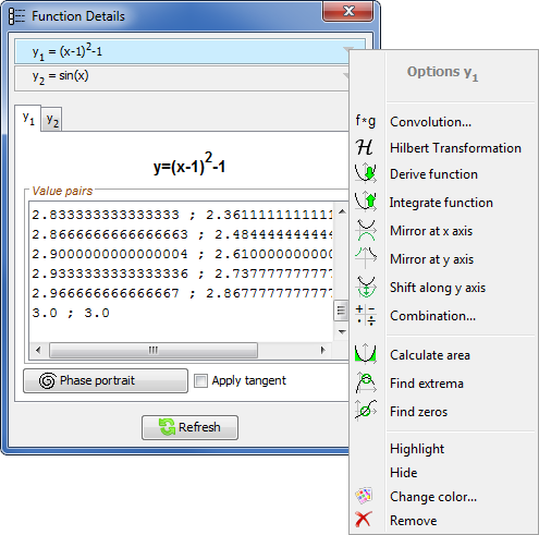
Details window
| The details menu automatically opens when after the first function has been added. With the menu item Details... the window can be opened manually. There can only be one instance of the details window. | 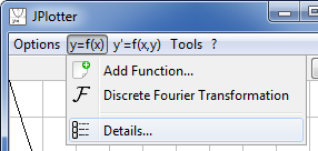 |
The details window provides details about all functions currently plotted. The details window is structured as follows:
| 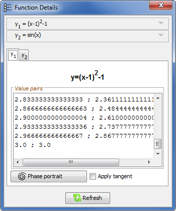 |
Plotting complex functions
The Options menu provides three different settings for the display of complex values:
| 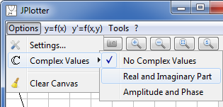 |
The difference between the modes can best be explained with the function `sqrt(x)` in the interval `[-5;5]`:
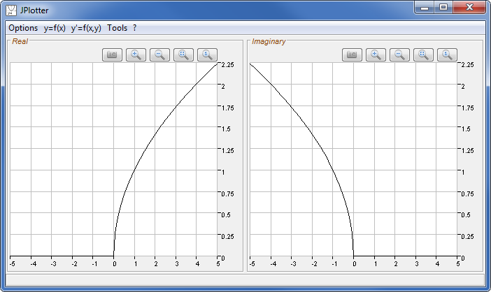
Real and Imaginary Part:
Since `sqrt(x)` with `x<0` in fact leads to complex numbers, the plotter automatically switches to this view. A complex function is defined as `f(x)=Re{f(x)}+i*Im{f(x)}` where `Re{f(x)}` and `Im{f(x)}` are real and imaginary part of `f(x)` and `i` is the imaginary unit.`Re{f(x)}` and `Im{f(x)}` are both real functions and can be plotted separately.
`sqrt(x)={(sqrt(x)+i*0,if x>=0),(0+i*sqrt|x|,if x<0):}` therefore `Re{sqrt(x)}={(sqrt(x),if x>=0),(0,if x<0):}` and `Im{sqrt(x)}={(0,if x>=0),(sqrt|x|,if x<0):}`
For `x<0` the real part is `0`. The imaginary part is `sqrt|x|`. For `x>=0` the real part becomes `sqrt(x)` and the imaginary `0`.
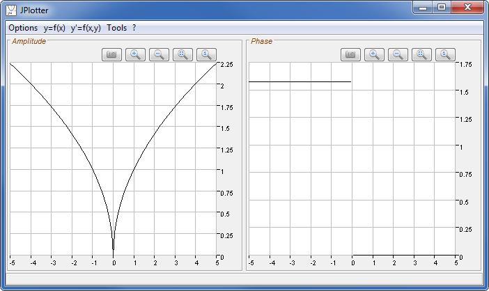
Amplitude and Phase:
Alternatively a complex function can be represented as `f(x)=|f(x)|*e^(i*arg(f(x)))` where the absolute value (amplitude) is `|f(x)|=sqrt(Re{f(x)}^2+Im{f(x)}^2)` and the phase (argument) is `arg(f(x))=arctan((Im{f(x)})/(Re{f(x)}))`.Again `|f(x)|` and `arg(f(x))` are two real functions which can be plotted separately.
`|sqrt(x)|={(sqrt(sqrt(x)^2+0^2)=sqrt(x),if x>=0),(sqrt(0^2+sqrt|x|^2)=sqrt|x|,if x<0):}` and `arg(sqrt(x))={(arctan(0/sqrt(x))=0,if x>=0),(arctan(sqrt|x|/0)=arctan(oo)=pi/2,if x<0):}`
The amplitude goes over the complete interval and is mirrored at the y-axis. For `x<0` The phase is `pi/2` because the imaginary part is non-zero while the real part equals zero. For `x>=0` the phase is `0` (as for normal real numbers).
No Complex Values:
| With complex numbers disabled the part of the function with complex numbers cannot be plotted.
So for `x<0` the values are NaN (not a number): `sqrt(x)={(sqrt(x),if x>=0),(text{undefined},if x<0):}` | 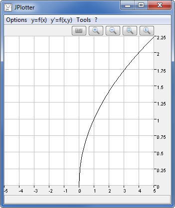 |
Example: RCR circuit
| The imaginary unit `i` can be directly used in the function
Let our complex function be `(1+i*x)/(1+2*i*x)` This is the system equation of a RCR system: 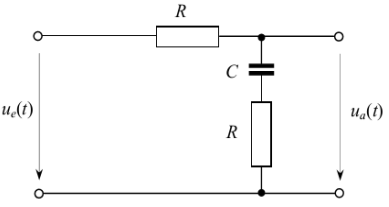
(where `R=2` and `C=1/2`). |  |
The math behind it:
where `sqrt((1+x^2)/(1+(2x)^2))` is the amplitude function and `arctan(x)-arctan(2x)` is the phase function. Those two functions are real now. If you plot them separately you will get the same graphs as above.
Discrete Fourier Analysis
`X_k=sum_(n=0)^(N-1)x_n*(cos(-2 pi k n/N)+i*sin(-2 pi k n/N))` for point number `k` of a total of `N` function points (`k,N in ZZ`).
|
The Discrete Fourier Analysis is enabled with the menu item within the menu y=f(x).
This is a global option for all functions. The option can either be enabled or disabled. Assume we have two functions plotted with the interval `[0;2 pi]`: `y_1=sin(x)` `y_2=cos(x)` | 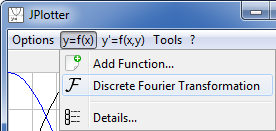 |
The resulting plot is:
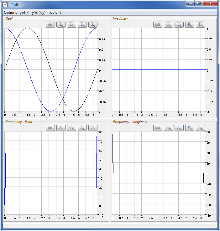 |
The upper two plots show real and imaginary part of the functions (DFT forces the display of complex numbers). The imaginary part the functions equals 0, since both functions are real. The lower two plots show real and imaginary part of the Fourier transforms. The color of the Fourier function equals the color of the original function. |
Fourier transform is real only with two positive peaks at the beginning and ending of the interval.
For `sin(x)`:
Fourier transform is imaginary only with one positive peak at the beginning and one negative peak at the ending of the interval.
The math behind it (for continuous functions):
`F{f(x)} = 1/(sqrt(2 pi)) * int_-oo^oo f(x)*e^(-i omega x) dx`
`F{sin(x)} = F{1/(2 i) (e^(i x) - e^(-i x))} = 1/(sqrt(2 pi)) * int_-oo^oo 1/(2 i) (e^(i x) - e^(-i x))*e^(-i omega x) dx = 1/(2 i sqrt(2 pi)) * int_-oo^oo (e^(-i x (omega - 1)) - e^(-i x (omega + 1))) dx`
`F{sin(x)} = 1/(2 i sqrt(2 pi)) * (delta(omega - 1) - delta(omega + 1)) = i/(2 sqrt(2 pi)) * (delta(omega + 1) - delta(omega - 1))`
The resulting function is imaginary-only with `delta` being the two Dirac impulses (one positive, one negative).
`F{cos(x)} = F{1/2 (e^(i x) + e^(-i x))} = 1/(sqrt(2 pi)) * int_-oo^oo 1/2 (e^(i x) + e^(-i x))*e^(-i omega x) dx = 1/(2 sqrt(2 pi)) * int_-oo^oo (e^(-i x (omega - 1)) + e^(-i x (omega + 1))) dx`
`F{cos(x)} = 1/(2 sqrt(2 pi)) * (delta(omega - 1) + delta(omega + 1))`
The resulting function is real-only with `delta` being the two Dirac impulses (both positive).
For further examples on DFT see rectangle / unity step function and Dirac Impulse in the following section.
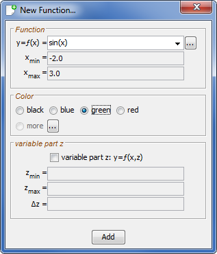
Function wizard
| The function wizard allows for adding special functions and provides templates for easier creation of
mathematical functions f(x). The template Parabola was initially a test for the template functionality. The parabola equation can directly be typed into the function text field without the use of this wizard. The Any Function template provides a list of all mathematical functions supported from which any custom function f(x) can be built. However once the syntax and the available functions are known the desired function f(x) can also directly be typed into the function text field without the use of this wizard. | 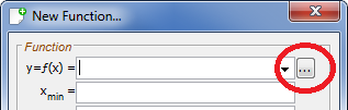 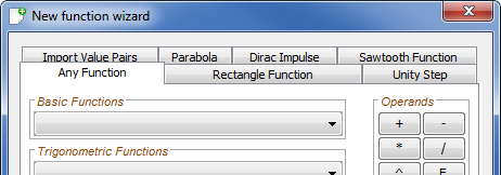 |
Rectangle, Sawtooth, Unity step function:
Rectangle, Sawtooth and Unity step function are basic functions for signal processing. Due to their characteristics they are often used as input for signal processing systems or being combined with other functions.These functions can only be added by the use of the wizard. There is no way of typing them as a f(x) function.
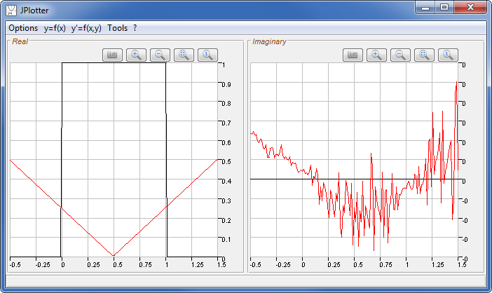
Example of a non-periodic rectangle function with Discrete Fourier Analysis:
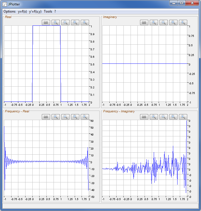 | Rectangle function with the following properties:
The real DFT part is a high-frequent si-function (`si(x)=sin(x)/x` starting from left to middle, then another interval starts). The imaginary DTF part is basically zero. Rounding errors cause a noisy function. However the y-axis scale displays all zeros. |
Let's check the inverted case:
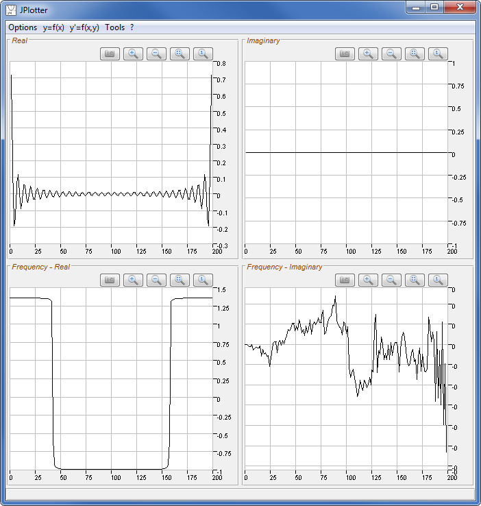 | High-frequent si function `si(x)+si(x-200)` within `[0;200]`. The DFT is a rectangle again. Since `F{F{f(x)}} = f(-x)` the rectangle is inverted. The imaginary part again is a noise function caused by rounding errors. |
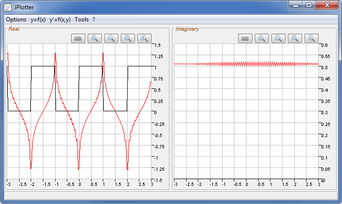
Example of a periodic sawtooth function and unity step functions:
 | The plot shows:
|
Example of a unity step function with its Discrete Fourier Transform:
Dirac Impulse:
The Dirac Impulse (also Delta Distribution) is another important signal used for describing signal processing systems. The following plot shows the Dirac Impulse with its Fourier Transform: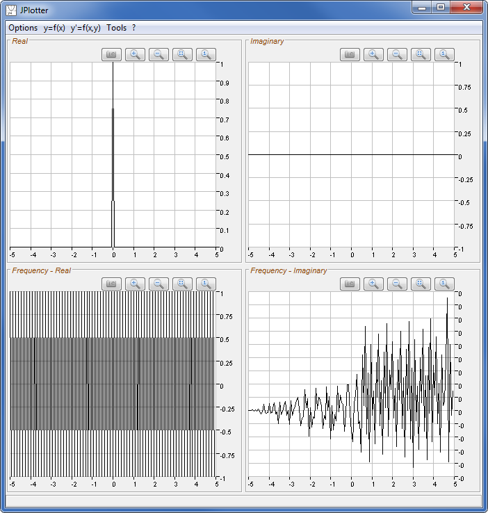 | The Dirac Impulse is a very short pulse of theoretically infinite height. The Dirac Impulse contains all frequencies over the complete domain. The imaginary part again is a noise function caused by rounding errors. |
Interpolation of points:
The wizard template Import Value Pairs allows for creating a function that interpolates a set of points (x/y value pairs). Different interpolation techniques are supported.| Example: Interpolation of 8 points:
| 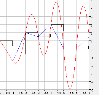 | Three interpolation techniques are displayed:
Other techniques are:
|
Hints for the input:
- In the wizard text area the value pairs must be comma separated (as in the example above).
- One point (x/y pair) each line.
- Spaces will be removed.
- By importing a csv file, the first column will be interpreted as x value, the second as y value. Additional columns will cause paring errors.
- Lines that cannot be parsed will be ignored, as long as at least one line was parsed successfully.
- Complex numbers are not (yet) supported for interpolation.
Function options
 |
The options are:
|
Convolution:
The convolution of two functions `f(x)` and `g(x)` is defined as: `{f(x)}**{g(x)} = F{F^-1 {f(x)} * F^-1 {g(x)}}`.Example:
 |
Rectangle function with the following properties:
Convolution with itself: The resulting function is a triangle function (real part). The imaginary part is noise, caused by rounding errors in the DFT. |
Hilbert Transformation:
The Hilbert Transformation of a function `f(x)` is defined as: `H{f(x)} = f(x) ** 1/(pi x)`. The convolution theorem allows: `H{f(x)} = F{f(x)} * (-i * sig(x))` with `sig(x) = {(1,if x>0),(0,if x=0),(-1,if x<0):}`.Example:
 |
Rectangle function with the following properties:
Hilbert Transformation in red. Due to rounding errors caused by the DFT the resultung function contains some noise. The imaginary part is theoretically constant. |
Derive Function:
The derivative of a function is defined as `f'(x) = d f(x) / dx`. With the sample points of a function the derivative is approximately `f'(x_n) = (f(x_(n+1)) - f(x_n)) / (Delta x)`. Thus the derivative shows the slope of the base function.Some examples:
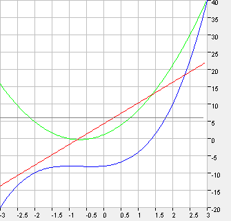 |
`y_1 = x^3 + 2 x^2 + x - 8` `y_2 = y_1' = 3 x^2 + 4x + 1` `y_3 = y_2' = y_1'' = 6x + 4` `y_4 = y_3' = y_1''' = 6` |
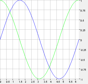 |
`y_1 = sin(x)` `y_2 = y_1' = cos(x)` |
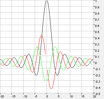 |
`y_1 = si(x) = sin(x)/x` `y_2 = y_1' = (cos(x) * x - sin(x)) / x^2` `y_3 = y_2' = y_1'' = (-x^2 * sin(x) - 2x * cos(x) + 2 sin(x)) / x^3` |
||
Integrate Function:
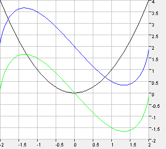
The primitive (or antiderivative) `int f(x) dx` of a function `f(x)` is defined such that `(int f(x) dx)' = f(x)`. Since an infinite number of primitives belong to the same derivative (this is because scalar numbers, which mean the shift along the y-axis, are dropped when derived), a base number `f(x_min)` has to be specified for integrating. This is the first y value at `x_min`.Example:
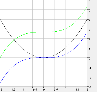 |
`y_1 = x^2` within `[-2 ; 2]`
Mathematically: `int x^2 dx = 1/3 x^3 + C` `y_2 = int y_1 dx` with `f(x_min) = f(-2) = 0` to determine `C`: `f(-2) = 0 = 1/3 (-2)^3 + C => C = 8/3`. `y_3 = int y_1 dx` with `f(x_min) = f(-2) = -8/3` to determine `C`: `f(-2) = -8/3 = 1/3 (-2)^3 + C => C = 0`. |
How does integrating work?
- the first y value is: `y_0 = f(x_min)` as specified by the user
- all following y values: `y_n = (f(x_(n-1)) + f(x_n)) / 2 * Delta x + y_(n-1)`
Mirror Function:
|
Mirror at x-axis: Any function plotted can be mirrored at the x-axis. The resulting function is `-f(x)`. Of cause manually added functions can be mirrored manually by just adding the same function with prefix '-'. However resulting functions (such as derivatives, Fourier transform, Hilbert transform, ...) can be mirrored by use of this option. | 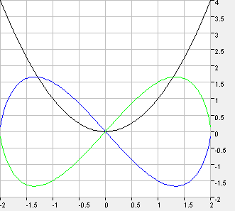 |
Example: `y_1 = x^2` `y_2 = H{y_1}` (Hilbert transformation) `y_3 = -y_2 = -H{y_1}` |
|
Mirror at y-axis: Original user functions can be mirrored at the y-axis. The resulting function is `f(-x)`. However this option is not available for resulting functions (such as derivatives, Hilbert transform, ...). This is because resulting functions are calculated based on another function and mirroring would require data which is not there. For user functions `x` can be replaced by `-x` to aquire mirroring. | 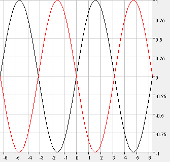 |
Example: `y_1 = sin(x)` `y_2 = sin(-x)` |
In case of complex functions:
Shift Function:
Any function plotted can be shifted along the y-axis. The resulting function is `f(x) + Delta y`. Of cause manually added functions can be shifted manually by just adding `Delta y` to the function. However resulting functions (such as derivatives, Fourier transform, Hilbert transform, ...) can be shifted by use of this option.Example:
 |
`y_1 = x^2`
`y_2 = H{y_1}` (Hilbert transformation) `y_3 = y_2 + Delta y` (with `Delta y = 2`) |
Combine Function:
Any function plotted can be combined with another function. Possible operations are addition, subtraction, multiplication and division.Examples:
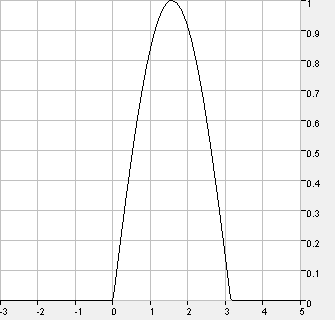 |
`y_1`: rectangle: `y_max = 1; y_min = 0; Delta x_1 = pi; Delta x_2 = pi;` non-periodic (single pulse);
function is hidden `y_2 = sin(x)`; function is hidden `y_3 = y_1 * y_2` the result is one single sine pulse. |
 |
`y_1`: delayed unity step: `y_0 = 0; A = 1; Delta x = -1`;
function is hidden `y_2 = x^2`; function is hidden `y_3 = y_1 * y_2` the result is a parabola which starts at -1. |
Area Calculation:
JPlotter can approximate the area between two functions or between one function and the x-axis.Examples:
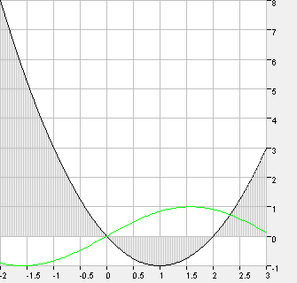 | Area between `x^2-2x` and the x-axis within `[-2;3]`: `~~ 9.333`
Let's check: `A = int_(-2)^0 (x^2-2x)dx + |int_0^2 (x^2-2x)dx| + int_2^3 (x^2-2x)dx` `A = [1/3 x^3-x^2]_(-2)^0 + |[1/3 x^3-x^2]_(0)^2| + [1/3 x^3-x^2]_(2)^3` `A = -(1/3 (-2)^3-(-2)^2) + |1/3 2^3-2^2| + (1/3 3^3-3^2-(1/3 2^3-2^2))` `A = -(-8/3-4) + |8/3-4| + (27/3-9-(8/3-4))` `A = 20/3 + 4/3 + 4/3 = 28/3 ~~ 9.333` |
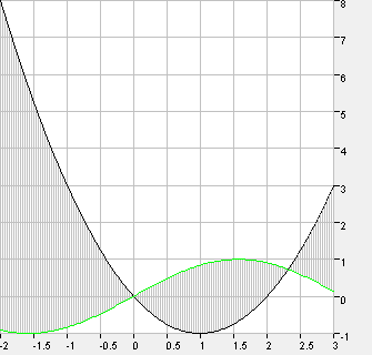 | Area between `x^2-2x` and `sin(x)`: `~~ 11.89` |
How does area calculation work?
The area calculation between a function and a derivative is less precise because the derivative function is always one sample shorter than the original function.
Keep in mind that this way areas are always positive! For example the area of `sin(x)` from `-pi` to `pi` is `2` and not `0`.
Find Extrema / Zeros:
JPlotter can approximately find extrema (minima or maxima) and zeros (roots) of any function plotted. The results are determined grafically. Potential complex complex results cannot be taken into account.Example: `y=e^-x * sin(10x)` within `[0; 5]`:
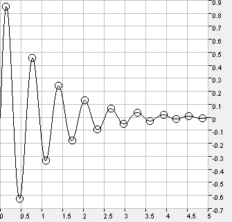 |
Extrema: Minima:
Maxima:
|
 |
Zeros (function crosses x-axis):
To calculate the zeros of a polynomial (also complex zeros) see the Calculate Zeros tool. |
Plot options
| The difference between a plot and a function is, that a plot is always a two-dimensional graph. So a function
can have one or two plots (e.g. real and imaginary part). The plot options are not among the function options but below the list of value pairs in the Details window. |
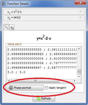 |
Apply a tangent on a function:
| Check box Apply tangent on the desired plot tab. Moving the cursor over
the canvas will apply a tangent at this very position. Click on the left mouse button will add the current tangent as a permanent function. | 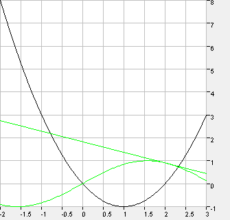 |
Example: Tangent on `sin(x)` at `x ~~ 2`. |
Phase Portrait:
A phase portrait of a plot is the slope (at y-axis) as a function of the y value (at x-axis). This can be a little hard to comprehend, but the following examples will help.Since phase portraits are no 'real' functions (in a mathematical manner) and slope (on y-axis) / y value (on x-axis) do not fit into a normal x/y coordinate system, they are always plotted in a separate window.
Example 1: phase portrait of `y=sin(x)` within `[0 ; 2 pi]`
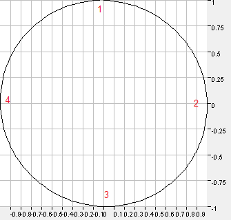 | The result is obviously a circle. Lets understand why: The sine at `x=0` starts with a high positive slope but the y value is 0. Remember that y value is on the x-axis and slope is one the y-axis. This leads to point 1. Til `x=pi/2` the y value of sine increases while the slope decreases. At `x=pi/2` the y value is at its max value of 1, while the slope is 0. This leads to point 2. Then the y value of sine starts to fall as the slope turns negative. At `x=pi` the y value of sine is 0 while the slope has its max negative value (point 3). Then to `x=3pi/2` the slope decreases (while still negative) til 0 while the y value reaches its max negative value of -1 (point 4). The sine completes its period until `x=2pi` while the slope starts to increase again and the y value develops to 0. This is again at point 1. |
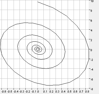 | The result is obviously a spiral, going from the edge to its center. Based on example 1 with the sine this is easy to understand. Basically we have a circle, too. But since the y value (and the slope as well) of the original function decreases each period the circle is a spiral becoming smaller and smaller. |
Plotting directional fields
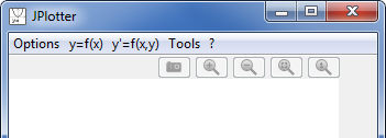
| The menu y'=f(x,y) allows for plotting of directional fields of differential equations. The required form is explicit form, first order: `y'=f(x,y)`. That means that each point `[x,y]` is assigned a slope `y'`. The slopes can be plotted as little lines. | 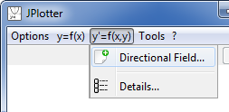 |
| In the following example the differential equation `y'=x*y` will be plotted.
As the area to plot we choose `[-1;-1]` to `[1;1]`. The resulting plot is: 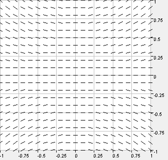 | 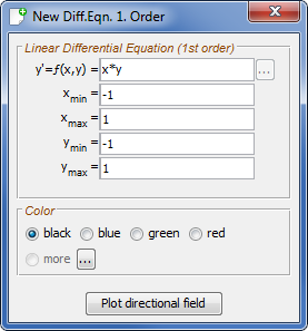 |
Let's look at the math for an analytical solution:
It seems the slope lines represent some kind of parabolic function (similar to `x^2`).
|
If we assume an initial value `[0;1]` `C` can be calculated: `1 = C * e^(0) = C` and the solutions becomes
`y=e^(1/2*x^2)`.
Now this function can be added to the canvas as a simple real function (menu y=f(x), notation: e^(0.5*x^2) ). As you can see the course of the red function (which is the solution of the differential equation with initial value `[0;1]`) pretty much matches the course of certain slope lines. Once again this is because the slope lines lead to the courses of all possible solution functions and the red function is the one particular solution which matches the initial value. | 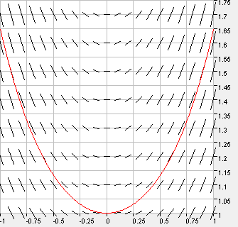 |
How does plotting of directional fields work?
The slope can be plotted as a little line with the function `slope * x`.
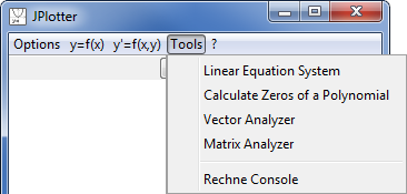
Tools
The Tools menu provides different tools for mathematical calculations:
|  |
Solve Linear Equation Systems:
By the use of the Gauss algorithm any linear equation system can be solved.Some examples:
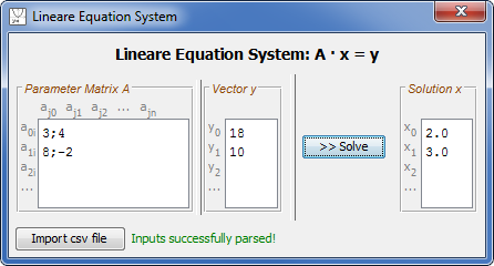 | `((3,4),(8,-2)) * vec x = ((18),(10))`
Solution: `vec x = ((2),(3))` |
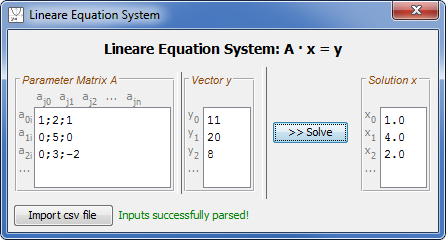 | `((1,2,1),(0,5,0),(0,3,-2)) * vec x = ((11),(20),(8))`
Solution: `vec x = ((1),(4),(2))` |
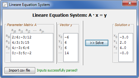 | `((2,6,-3,12),(4,3,3,15),(4,-3,6,6),(0,-3,5,-2)) * vec x = ((-6),(6),(6),(14))`
Solution: `vec x = ((-3),(2),(4),(0))` |
- Separation by comma and line break (as in the examples above).
- Spaces will be removed.
- The parameter matrix A must always be a square matrix. The vector y must always have the same lenght as the matrix.
- By importing a csv file, the first columns will be interpreted as the matrix A, the last column as y vector. Thus the csv file must have the correct dimension: n+1 columns, n rows. Additional columns/rows will cause parsing errors.
- Values that cannot be parsed will be highlighted.
- Complex numbers are not (yet) supported.
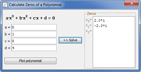
Calculate Zeros (Roots) of a Polynomial:
The zeros (roots) of a polynomial up to 3rd order can be calcualted numerically. The difference to the Find Zeros function option is, that not only real zeros (cross with x-axis) will be determined, but also complex zeros as each polynomial has always the number of analytical zeros as its order.Some examples:
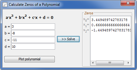 | `y = 3x^3 - 8x^2 - 11x + 10`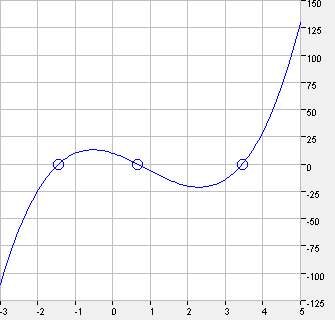 |
3 real zeros: `x_0 = 1+sqrt(6) ~~ 3.45` `x_1 = 2/3 ~~ 0.66` `x_2 = 1-sqrt(6) ~~ -1.45` |
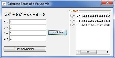 | `y = x^3 + x^2 + x + 1`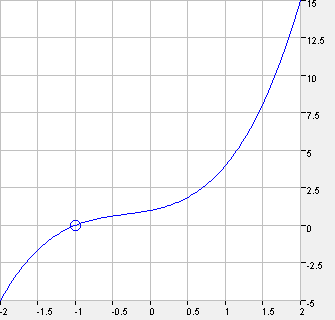 |
1 real, 2 complex zeros: `x_0 = -1` `x_1 = i` `x_2 = -i` Due to rounding errors the displayed results differ from the exact results. |
 | `y = x^2 + 4`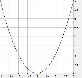 |
2 complex zeros: `x_0 = 2i` `x_1 = -2i` Proof: `0 = x^2 + 4 -> -4 = x^2` `x = +- sqrt(-4) = +- 2i` |
Analyze a Vector:
Different operations can be performed on an input vector (complex values allowed). The operations are:- DFT: Discrete Fourier Transformation (see also section DFT). The result is a vector `F{vec x}` of the same lenght.
- Inverse DFT: inverse Discrete Fourier Transformation. The result is a vector `F^-1 {vec x}` of the same lenght.
- Different vector norms. The result for each norm is a real number.
Examples:
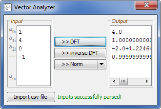 | `F ((1),(4),(0),(-1)) = ((4),(1+5i),(-2),(1-5i))` `F^-1 ((1),(4),(0),(-1)) = ((1),(1/4-5/4i),(-1/2),(1/4+5/4i))` | Maximum norm: `max|x_i| = 4`
Row sum norm: `sum_(i=1)^n |x_i| = 6` Euclidic norm: `sqrt(sum_(i=1)^n x_i ^2) = sqrt(18) ~~ 4.24` |
| The following vector represents 4 samples of the sine function. For comparison see section
DFT for the graphical Fourier analysis of `sin(x)`. The result is one positive and one negative
imaginary peak. | ||
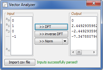 | `F ((0),(1),(0),(-1)) = ((0),(2i),(0),(-2i))` `F^-1 ((0),(1),(0),(-1)) = ((0),(-1/2i),(0),(1/2i))` | Maximum norm: `max|x_i| = 1`
Row sum norm: `sum_(i=1)^n |x_i| = 2` Euclidic norm: `sqrt(sum_(i=1)^n x_i ^2) = sqrt(2) ~~ 1.41` |
- Separation of vector elements by line break (column vector).
- Spaces will be removed.
- Complex values in the form: '1+2*i'
- By importing a csv file, only ONE column is allowed. Additional columns will cause parsing errors.
- Values that cannot be parsed will be highlighted.
Analyze a Matrix:
Different operations can be performed on an input matrix (real values only). The operations are:- Calculate the determinant of a square matrix. The result is a real number.
- Calculate the Eigen values of square matrices up to size 3. The result is a vector of the Eigen values (number of Eigen values equals dimension of the matrix: 2 or 3).
- Invert a square matrix. The result is a new matrix of the same size.
- Different matrix norms. The result for each norm is a real number.
Example:
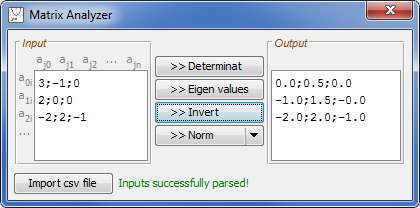 Eigen values: `det((3-lambda,-1,0),(2,-lambda,0),(-2,2-lambda,-1)) = 0 => {: (lambda_0=2),(lambda_1=1),(lambda_2=-1) :}` Determinant: `det A = -2` | `A = ((3,-1,0),(2,0,0),(-2,2,-1)) => A^-1 = ((0,1/2,0),(-1,3/2,0),(-2,2,-1))`
Norms:
|
Hints for the input:
- Separation by comma and line break (as in the example above).
- Spaces will be removed.
- The input must always be a square matrix.
- By importing a csv file, the number of columns must equal the number of rows (square matrix!). Additional columns/rows will cause parsing errors.
- Values that cannot be parsed will be highlighted.
- Complex numbers are not (yet) supported.
- Calculation of Eigen values only supported for matrices of size 2 or 3.
Rechne Console:
Rechne Console is a pocket calculator and frontend for the rechne.exe library.Some Examples: | 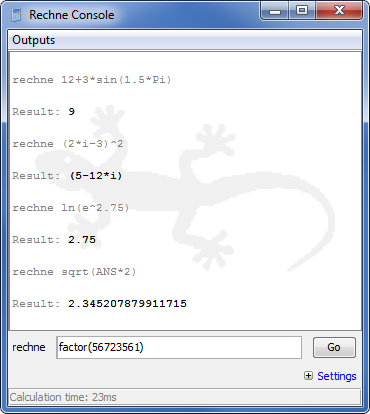 |
- Verbosity: if checked all intermediate calculation steps are displayed.
- Transfer between different numerical systems (e.g. decimal numbers to binary numbers; hexadecimal to decimal; ...)
- Precision: automatic (scientific display of numbers, use of E if appropriate), rounding to a fixed number of decimal places or rounding to integers.
List of functions/operations:
| modulus | mod | factorial | fac | raising | ^ |
| shift decimal point | E | root | rt | square root | sqrt |
| logarithm | log | natural logarithm | ln | decimal logarithm | lg |
| binary logarithm | ld | parallel operation | // | binominal coefficient | binom |
| sinc function | si | sine | sin | cosine | cos |
| tangent | tan | secant | sec | cosecant | csc |
| cotangent | cot | arcsine | asin | arccosine | acos |
| arctangent | atan | arcsecant | asec | arccosecant | acsc |
| arccotangent | acot | hyperbolic sine | sinh | hyperbolic cosine | cosh |
| hyperbolic tangent | tanh | hyperbolic cotangent | coth | area hyperbolic sine | asinh |
| area hyperbolic cosine | acosh | area hyperbolic tangent | atanh | area hyperbolic cotangent | acoth |
| numerical integral | sum | product integral | prd | definite integral | int |
| random number | rand | fibonacci sequence | fib | signum function | sig |
| round-down | floor | round-up | ceil | real part | creal |
| imaginary part | cimg | absolute value | cabs | polar angle | carg |
| greatest real number | max | smallest real number | min | greatest magnitude | maxc |
| smallest magnitude | minc | greatest common divisor | gcd | least common multiple | lcm |
| factorization | factor | previous result | ANS | Pi | Pi |
| Eulers number | e | imaginary unit | i |
License
Please note: As stated in GPL JPlotter comes with absolutely no warranty.
rechne.dll and sources from the rechne.exe project are GPL as well.